

For various reasons biking is becoming a more frequently used mode of transportation. It offers flexibility, is quite cheap compared to other modes of transportation, helps with fitness and is almost carbon neutral. To evaluate how well adapted the existing infrastructure is to accommodate biking, Manuel Kraft of HeiGIT created the “Bikeability-Index”.
Analyzing Bikeability
There are multiple definitions in scientific literature for the term ‘bikeability’. According to Gehring it describes the suitability of cycling by considering several properties of the constructed environment that are capable of promoting or hindering cycling (Gehring 2016).
There are many approaches to calculating the index. In most cases geographic data is retrieved from different sources that are not always accessible for the public. Heinemann used a different approach in her bachelor thesis (Heinemann 2022). Her analysis of bicycle friendliness in Heidelberg relies entirely on open source OpenSteetMap (OSM) data (ibid.).
Within this workflow, the bachelor thesis of Heinemann will be used as a template. Many assumptions made by her are integrated as parameters, especially five bikeability indicators that compose the bikeability index.
However, there are three main improvements in contrast to the origin analysis:
- The workflow is entirely automatized with R and Python (preparing, downloading, editing, calculating).
- The calculation can be done for multiple timestamps all at once. The adapted classification standardizes the bikeability index values which enables them to be compared by region and by timestamp.
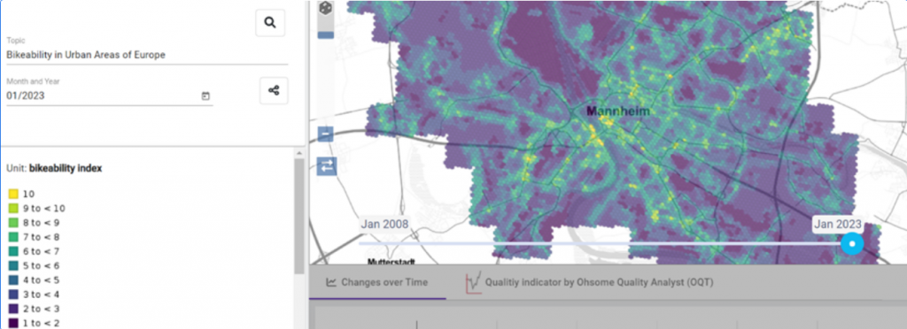
- The Index is calculated only for urban areas that are included in the Global Human Settlement Layer as the chosen bikeability indicators are not suitable for rural areas (Airaghi et al. 2019). The results will be visualized in ohsome-hex by hexagons (Figure 1). The index values range from 1 (weak bikeability) to 10 (strong bikeability).
In the following chapters a brief outline of the workflow is given.
2. Indicators
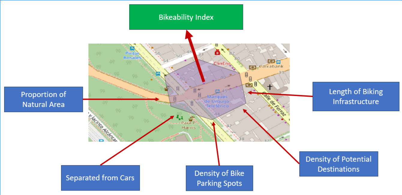
According to Heinemann (2022) the Bikeability Index is composed of five indicators:
- Length of biking infrastructure: meters within 250 meter buffer from hexagon centroid
- Proportion of natural area: area percentage within hexagon
- Density of bike parking spots: number within 100 meter buffer from hexagon centroid
- Density of potential destinations: number within 250 meter buffer from hexagon centroid
- Separated from cars: number within hexagon
Each hexagon cell contains the values of all five indicators (Figure 2). All of these indicators influence the final index in a positive way. Hence, the higher the natural area, longer the bicycle infrastructure, et cetera the higher the index. The Bikeability Index is the average of the indicators.

3. Classification
To derive a summarized value from all five indicator values, these values have to be classified to the same scale. The challenge of the classification is to derive an appropriate orientation value at which the indicator values are considered as „good“ (or 10 out of 10).
To do so, five regions are used as model regions:
- Copenhagen
- Utrecht
- Amsterdam
- Muenster
- Bremen alte Neustadt
These regions are known for their high bicycle friendliness (ADFC 2022; Luco Cover SAS 2022; Stadt Münster 2023; http://Copenhagenize.eu Design Co. 2019; bremen.online 2022).
The orientation value at which the indicator value is considered as “good” (or 10 out of 10) is obtained by analyzing the statistics of the indicator values from all five model regions. Therefore the choice of the model regions has a big impact on the final results.
A detailed explanation of how the orientation values are obtained and how the classification is done is publicly available on github: https://github.com/GIScience/osm-bikeability/blob/main/documentation.md .
4. Final Bikeability Index
The classified values for the five bikeability indicators can be summarized to the final bikeability index. The following example illustrates the calculation:
- Hexagon-ID: 3295746
- Timestamp: 2022-01-01
- Classified indicator values:
- Length of infrastructure: 2
- Proportion of natural area: 2
- Separated from cars: 1
- Density of potential destinations: 8
- Density of bike parking spots: 1
- Bikeability-Index: (2 + 2 + 1 + 8 + 1) / 5 = 2.8
→ The hexagon with the ID: 3295746 has got a bikeability value of 2.8 at the timestamp 2022-01-01
5. Discussion
The described analysis of the bikeability index enables a powerful comparison of the bikeability between timestamps and regions. Scientific literature is used as a template for thematic assumptions like the decision of appropriate indicators and the according OSM filters. Previous studies are extended by implementing an automated workflow to calculate the final index. Both, the data sources (OpenStreetMap, Global Human Settlement Index) and processing tools (Python, R, Ohsome-API, PostGis) are open source and enable simple replication.
However, there are some limitations that have to be mentioned. The fundamental data source is OSM and the calculation of the bikeability values already starts at 2008. In the early stages of OSM the mapping completeness was limited and therefore geographic objects that contribute to higher bikeability values were missing. An increase of bikeability values over time is dominantly caused by an increase of mapped geo-objects rather than an increase of real world bikeability.
Furthermore, suitable indicators for bikeability differ in literature and an overall common thinking within the scientific community is not yet detectable. Upcoming studies might falsify recent assumptions that are currently used.
Even if the chosen indicators depict real world bikeability in the best way, the representation of according OSM objects is still a challenge. OSM tags (or attributes) are not standardized and mappers can individually set uncommon attributes. That challenges the filter implementation as these filters rely on common (inofficially) standardized OSM tags. Inspecting the filters and reporting missing or outdated tags is always welcome and will improve the analysis.
It is also important to mention that OSM data is not suitable for all kinds of important information with regard to bikeability. For example, the analysis could strongly benefit from motor traffic intensity as the amount and the speed of driving motor vehicles definetely decrease the motivation to cycle. Unfortunately, road attributes about speed limits and motor vehicle frequency is barely available in OSM and extending the analysis with this bikeability indicator is not possible. However, extending the analysis with other data sources might solve this problem but that contradicts the general interest of open source based analyses.
6. Conclusion
The Bikeability-Index describes the suitability of cycling by considering several properties of constructed environment that are capable of promoting or hindering cycling (Gehring 2016). To calculate the Index, underlying thematic assumptions have to be made with regard to appropriate bikeability indicators and OSM filters. To do so, the previous study from Heinemann is used as a template (Heinemann 2022).
However, this analysis extends current calculations by implementing a mainly automatized workflow to calculate the index. Furthermore, the updated classification enables comparisons between multiple cities and timestamps.
Both, the data sources and the processing tools are open source and enable simple replication. Everything a user needs is an internet connection, the Global Human Settlement Layer (GHSL), an accessible postgis database, R and python.
The underlying assumptions for the calculations can still be modified and any suggestions are always welcome, especially with regard to the OSM filters and the classification method. Suggestions can be made by creating an issue within the attached repository or by mail (manuel.kraft@heigit.org).
Nevertheless, the current state of the analysis already increases knowledge of spatial bikeability distribution, both at a small scale within urban areas and at a high scale between european cities.
7. Sources
Allgemeiner Deutscher Fahrrad Club. (2022). Utrecht: In zehn Jahren zur Fahrradstadt der Superlative. Von https://www.adfc.de/artikel/utrecht-in-zehn-jahren-zur-fahrradstadt-der-superlative abgerufen
Barnes, R., & Sahr, K. (2017). dggridR: Discrete Global Grids for R. R package version 2.0.4. Von “https://github.com/r-barnes/dggridR/ abgerufen
bremen.online. (2022). Deutschlands erste Fahrradzone in Bremen. Wirtschaftsförderung Bremen GmbH. Abgerufen am 29. 08 2023 von https://www.bremen.de/leben-in-bremen/fahrradstadt-bremen/fahrradzone
http://Copenhagenize.eu Design Co. (2019). https://copenhagenizeindex.eu . Abgerufen am 29. 08 2023 von https://copenhagenizeindex.eu/the-index
European Commission. (2020). GHSL – Global Human Settlement Layer. (E. Commission, Herausgeber) Abgerufen am 01. 09 2023 von https://ghsl.jrc.ec.europa.eu/ghs_stat_ucdb2015mt_r2019a.php
Florcyk, A., Corbane, C., Schiavina, M., Pesaresi, M., Maffenini, L., Melchiorri, M., . . . Zanchetta, L. (2019). GHS-UCDB R2019A – GHS Urban Centre Database 2015, multitemporal and multidimensional attributes. Abgerufen am 29. 08 2023 von https://data.jrc.ec.europa.eu/dataset/53473144-b88c-44bc-b4a3-4583ed1f547e
Gehring, D. (2016). Bikeability-Index für Dresden – Wie fahrradfreundlich ist Dresden. Masterarbeit an der Professur für Verkehrsökologie, TU Dresden, Verkehrsökologie. Von http://nbn-resolving.de/urn:nbn:de:bsz:14-qucosa-201073 abgerufen
Heinemann, M. (2022). Radfreundlichkeit in der Stadt. Umsetzung eines Bikeability-Index auf Basis von OpenStreetMap am Beispiel Heidelberg. Heidelberg Institute for Geoinformation Technology, Geographie, Heidelberg.
Kraft, M. (2023). Bikeability. Von https://github.com/GIScience/osm-bikeability/tree/main abgerufen
Luko Cover SAS. (2022). Global Bicycle Cities Index 2022 – the most cyclist-friendly cities around the world, based on data. Abgerufen am 29. 08 2023 von https://de.luko.eu/en/advice/guide/bike-index/
Stadt Münster. (24. 4 2023). ADFC-Fahrradklima-Test: Münster belegt Spitzenplatz. Abgerufen am 29. 08 2023 von https://www.stadt-muenster.de/aktuelles/pm-details?1127264
All scripts and files that are referred to can be accessed via the following github repository:https://github.com/GIScience/osm-bikeability/tree/main (Kraft 2023).