

After introducing the OSM Element Vectorisation Tool earlier this week, we now want to show possible use cases and specific examples of what the tool can do. This first of three use cases takes a closer look at the data in the region of Heidelberg, Germany. We will use the concept of archetypes to identify a few contrastive elements. Please visit the repository for detailed information.
Archetypes
Archetypes in this context can be thought of as a group of elements that frame the population. One can think of them as the points that create a (multidimensional) convex hull around the data, but with a flexible number of edges. I.e. they mark the (multidimensional) extremes of a distribution. Therefore any element within the population can be described as a combination of the archetypes:
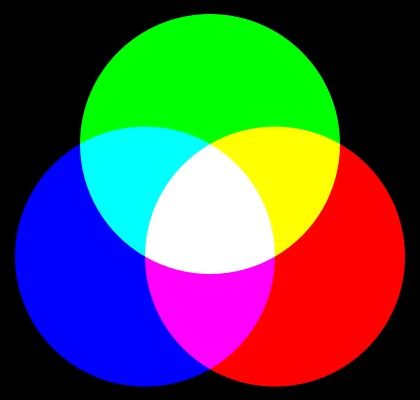
Figure 1: One of the simplest example of archetypes is the RGB colour spectrum with red, green and blue being the archetypes. All other colours are a certain combination of these archetypes. Image Source: Wikimedia Commons.
Archetypical objects, which are located at the edges of a distribution, are somehow the opposite of “typical” objects within the distribution. Therefore this analysis is similar to the paper by Peter Mooney and Padraig Corcoran (2012) where they look into the special case of the Characteristics of Heavily Edited Objects in OpenStreetMap.
Data
The data for this example covers the region of Heidelberg extracted on the first of January 2022 containing 8,838 elements. To reproduce this code, first download the example heidelberg from the API and convert it to a GeoPackage (see the README). For an overview of the exact implementation for the different data aspects, please refer to the documentation.
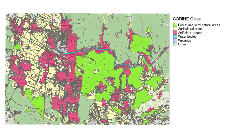
Figure 2: Overview of the data coloured by CORINE class. Blank spaces on the map either represent unmapped areas or the elements in these regions extend beyond the used bounding box and were therefore removed by the tool. The data represents a snapshot taken in 2022, which may become relevant later. Base layer: OSM Carto.
Preparation
Using the archetypes library we can get an estimation for a good choice for the number of archetypes:
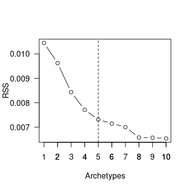
Figure 3: Screeplot of the residual sum of squares in relation to the number of archetypes chosen. The dashed line indicates the number of archetypes picked for the further analysis
As always with real data, the result of these helper functions is subject to interpretation and not as clear as most examples show. We will use the first noticeable knee of five archetypes (indicated by dashed line in the screeplot). For this high dimensionality, a larger number would of course be more fitting. Yet, already these five archetypes separate the data well into similar sized regions.
| Archetype | Nearest Neighbour Count |
|---|---|
| 1 | 2120 |
| 2 | 1856 |
| 3 | 1627 |
| 4 | 1406 |
| 5 | 1829 |
The method though not forcefully uses real data points to represent the archetypes. We will use the closest real data points (nearest neighbours) as an approximation for the given analyses.
To simplify the following plots we will crop the name of the elements to the significant part which in this case are the first two digits of the ID. Because IDs are given sequentially (by type), the order also orders the data by object age:
- way/68507169 -> 06
- way/97825572 -> 09
- way/107741432 -> 10
- way/285061545 -> 28
- way/838582144 -> 83
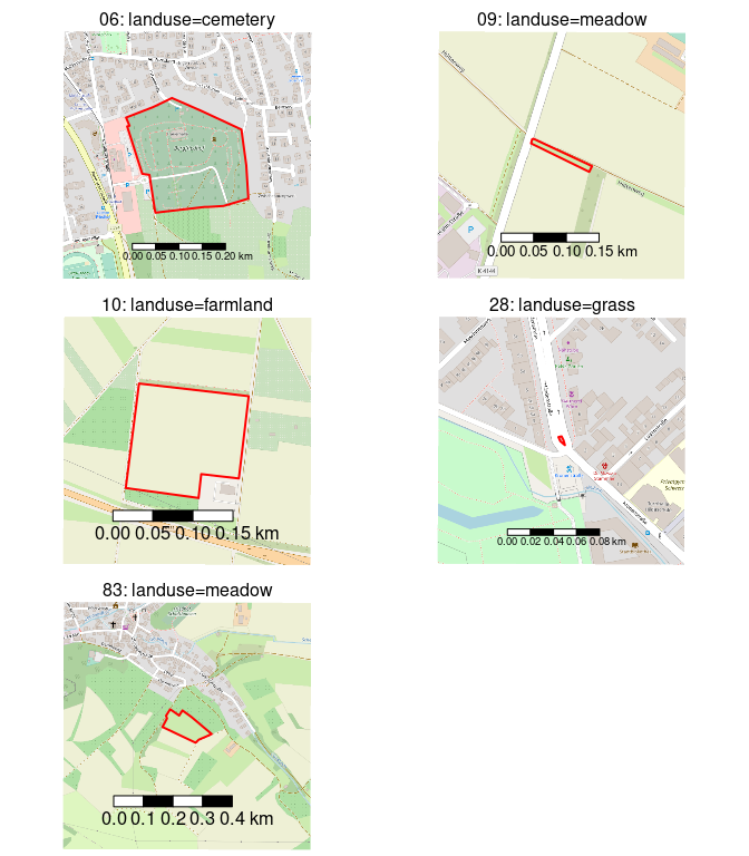
Figure 4: Detailed view on the five archetype objects.
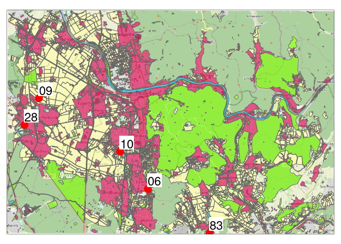
Figure 5: Location of the five archetype elements.
Investigation
All five elements are located on a west to south-east line. Which doesn’t mean anything1, but it sparks out. What is really interesting is that all five elements seem rather small. The natural order a human may apply (contrasting large and small objects) seemingly was not important for the algorithm to pick archetypes.
Looking at the linked websites, most objects were either mapped or touched by well known (local) power mappers like mike_hd, whb, zehpunktbarron, UE_Su, Paramida, Max– and mappy1232. This is equally expected information for anybody who knows that 90% of map edits are done by 10% or less of the community3. All of them represent green spaces or agricultural areas. But all this can be better expressed through the data itself.
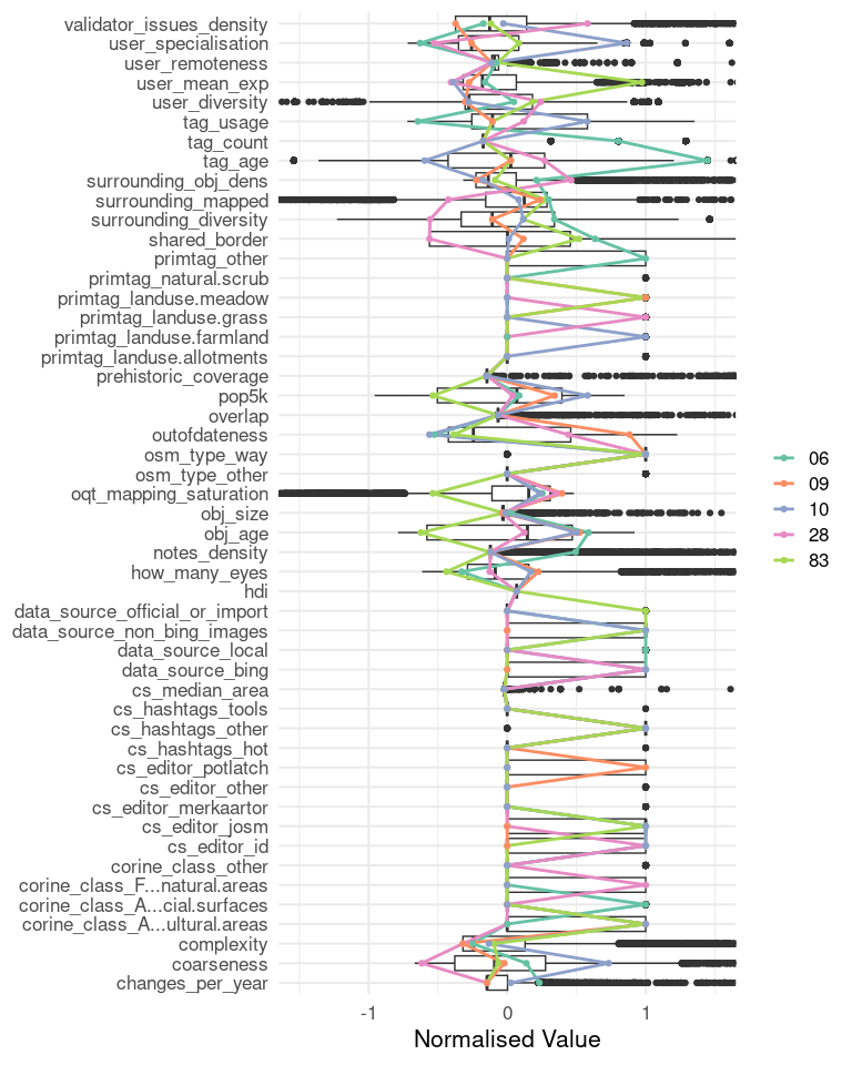
Figure 6: Attributes of the five archetypes in relation to the distribution within the dataset (boxplots).
We haven’t talked about the number of indicators we consider as we don’t want to get lost in the data just yet. We will choose six interesting attributes, but it is possible to adapt this choice later, e.g. when re-running the analysis. In fact, any of the examples should be sufficiently generic to be extended or re-run with different parameters. It is also possible to plug in other datasets that have been created using the OSM Element Vectorisation Tool.
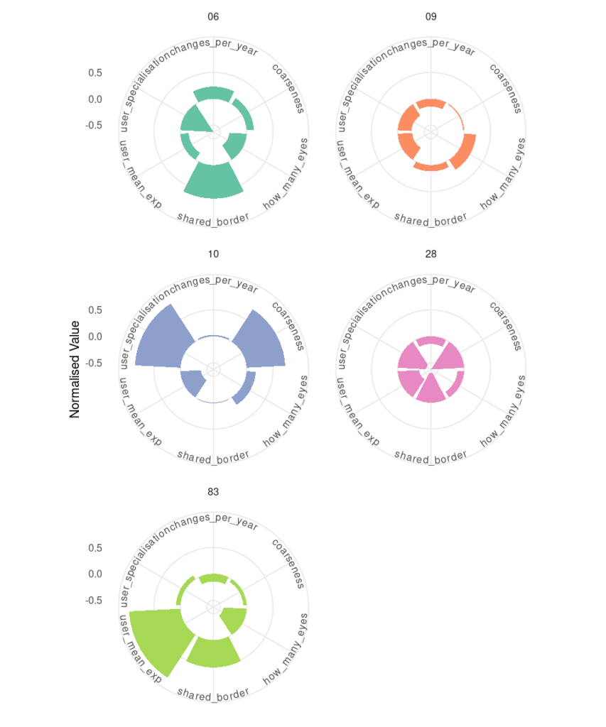
Figure 7: Selected characteristics of the five archetypes.
Combining all the information we have gathered so far we can characterise these elements quite nicely.
The oldest element (06), the cemetery in Leimen created in 2010, regularly receives changes and updates. It was created in a changeset that spans quite a large area but, according to the description, targeted this object specifically. The object has been changed seven times or once every two years in average since then. The high length of borders that it shares with neighbouring elements may be one reason, as changes to those elements may induce changes in this element as well. Another reason could be the size of the object which may seem small but in relation to the data distribution is in fact large. The bigger an element is, the higher the potential for changes may seem. Interestingly, the graveyard lies in an area with a relatively low number of unique mappers in relation to the amount of data present. So the assumption that many mappers lead to many updates is not true here. On average 1.2 users were active in this area every month to curate more than 500 OSM elements located here.
The farmland in Rohrbach (10), which is also one of the bigger elements, regularly received updates as well. It was (on average) only changed once every three years, which is close to the mean amount of changes in the whole dataset. This value is thought to be substantially higher than the number of changes that 75% of the data receives. In fact, many objects in OSM are never changed after creation. The farmland in Rohrbach is also interesting because it was created by an (at that time) highly specialised mapper. Max–, who at that time was already registered for two years but had only started their career, had created “only” 235 changesets so far (compared to >4,000 today). And seemingly many of their changes at that time were concentrated around the topic of land-use, hence the specialisation. Contrasting, the youngest element created in August 2020, which is the meadow in Kraichgau (83), was created by Paramida who at that time already had created more than 12,000 Changesets.
The smallest element in the set, the grassy traffic island in Schwetzingen (28), was created in May 2014 by chaostrooperwho is still active today. Yet they are not a “power mapper” and at that time only had mapped for ten days. Yet, they chose to map this very detailed object even though they were rather concentrated on highways and, to a lesser extend, buildings up until that point. It is therefore no surprise that this element was created in a changeset that referenced the update of the street network and seems to only have been a side product. All other objects were created in changesets that specifically referenced the land-use changes made therein.
As expected, each of the archetypes has at least one special feature, even the rather boring looking meadow in Schwetzingen (09). It is the only element in our small sample that was created using Potlatch. Potlatch was one of the first editors of OSM. It has since been rewritten two times and is still actively maintained in version 3 today.
Conclusion and Outlook
Choosing some elements at “random” and looking into their history and attributes can lead to interesting findings and helps to better understand the dataset as a whole. The archetype algorithm provided us with elements that were highly shaped by the core contributors of OSM in this region. Yet, the amount of information and the rate at which this information is interwoven make qualitative analyses time consuming. In the next example, we will therefore move away from a qualitative view to a more quantitative comparison between two regions.
1 It’s probably just because of the Odenwald forest in the north-east.
2 Due to the OSM data model, this of course only concerns major edits, meaning edits to the element itself. Changes to the underlying nodes are not reflected. For more information, see the OSHDB Documentation.
3 A rule described by Jacob Nielsen and since proven multiple times for OSM.