

The completeness of the OpenStreetMap (OSM) road network has been an ongoing focus for researchers for more than 15 years. For instance, Neis et al. (2011) investigated the OSM street network evolution in Germany and compared it against road data from TomTom. Whereas obtaining reference data has been rather difficult in the past, nowadays we observe that more and more datasets are released under an open data license. Sometimes these datasets are released by public mapping agencies, but increasingly, datasets derived through deep learning approaches, such as the Microsoft (MS) RoadDetections, are also becoming available and cover (almost) the entire globe.
Here, we want to report about our experiments to utilize the MS roads for OSM data completeness assessment. In particular, we will compare OSM road data with MS road data for selected cities and regions and test three different methodological approaches.
We downloaded data from MS roads from GitHub and from OSM using the ohsome API. For OSM we considered the following highway tag values: motorway, trunk, motorway_link, trunk_link, primary, primary_link, secondary, secondary_link, tertiary, tertiary_link, unclassified, residential, living_street, service, pedestrian, track, bus_guideway, escape, raceway, road, busway, path.
Results
Our results show that comparing OSM roads and MS roads is indeed not straight forward. Nevertheless, after a first visual inspection of the MS road data, it seems to be a good reference in cities for paved roads and could be used to estimate the amount of missing roads in OSM. In rural areas, especially in regions with many unpaved roads, the amount of misclassifications within the MS roads is much higher and the completeness estimation is less trustworthy.
Method 1: Length Comparison
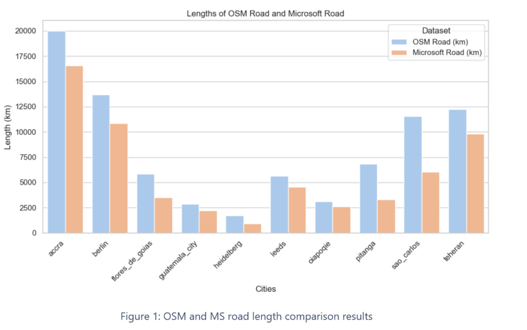
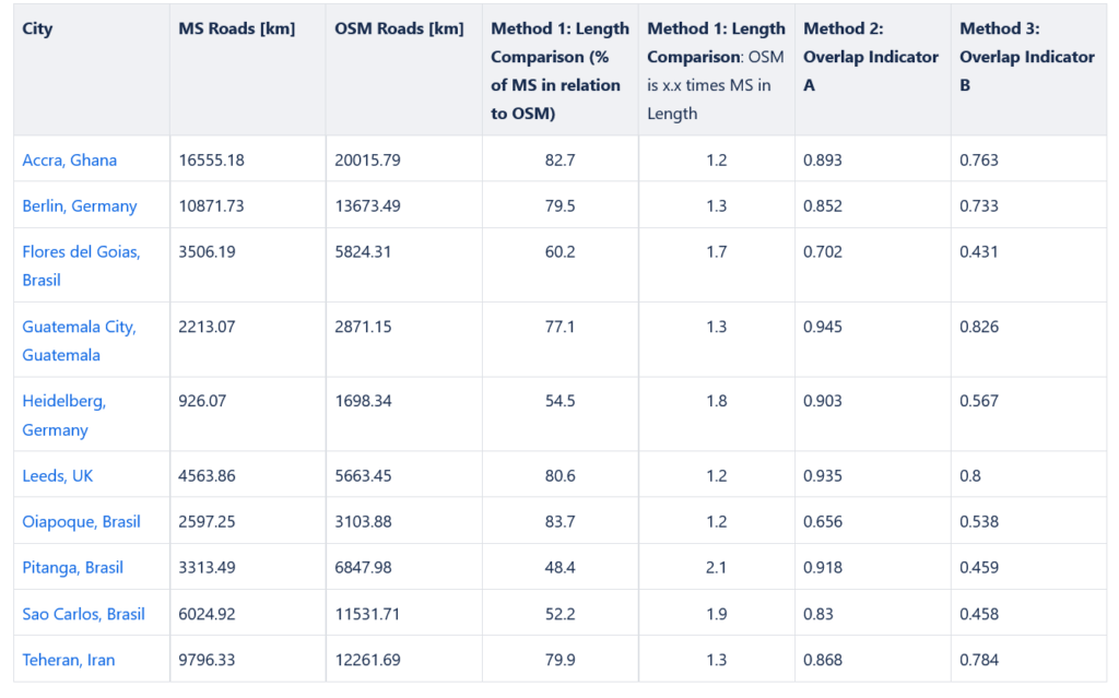
First, we conducted a simple comparison of the overall road length for both datasets. Interestingly, in all our study sites we found that the overall road length in OSM exceeded the road length in the MS dataset. For the case of Sao Carlos, Brazil the OSM road length is almost twice the length in the MS dataset.
To some extent this might be due to the fact that the OSM tags might not match the road types contained in the MS dataset. This seems to be the case for tracks and other minor roads which could be paved or not.
In general, this method seems to offer limited additional value for data quality estimation. Only for places where there is no OSM road data at all, the length comparison approach might offer some insights about the completeness of OSM road data.
Method 2: Overlap Indicator A
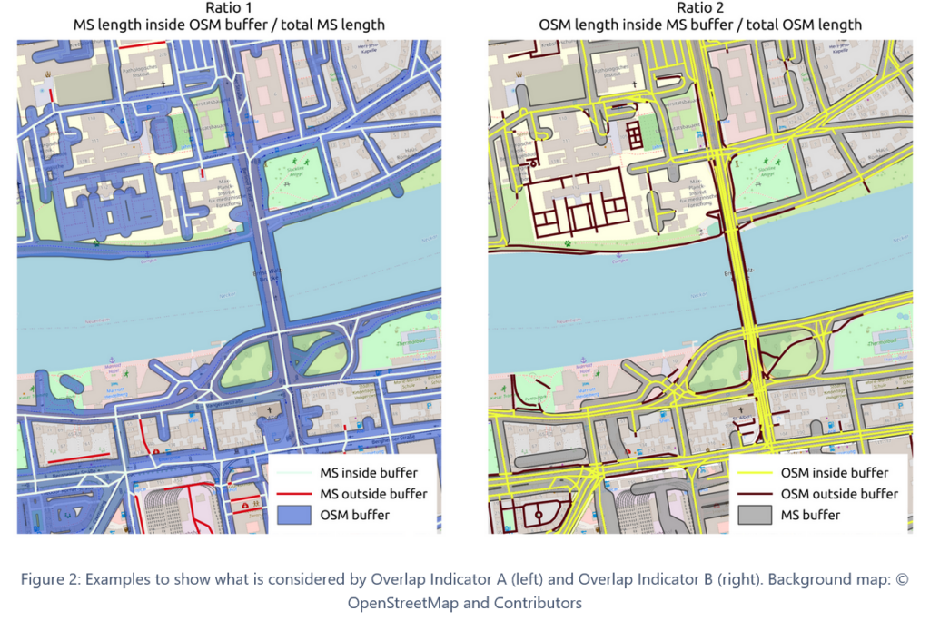
This method considers the spatial location of each road segment in the OSM dataset and investigates to what extent we find MS roads in the same location. In the Figure 2 below (left panel) the matching roads are in white and depict MS roads for which OSM roads are already mapped. The red roads represent all the roads which are not yet mapped in OSM. A high ratio indicates that there are only very few missing roads in OSM, which have been detected by MS.
Let’s take the example of Heidelberg: Here, OSM roads cover about 90.3% of the MS data. We can conclude that OSM is rather complete in comparison to the MS dataset. Still, this indicator also shows us that for Heidelberg about 9.3% of the MS roads are not yet mapped in OSM. In contrast, Flores de Goias, Brazil shows a much lower ratio of 70.2%. Here, we find that there are many road segments still missing from OSM. To some extent this might also be affected by the OSM tags considered in our analysis as we might unintentionally excluded some OSM data.
This Overlap Indicator method seems to be well suited to quantify missing data in OSM especially in cities. For rural areas it is more difficult to decide if roads missing in OSM are actually roads or rather misclassifications in the MS dataset.
Methods 3: Overlap Indicator B
This approach works similarly (but differently!) to the one described before. Here we consider the spatial location of each road segment in the MS dataset and investigate to what extent we find OSM roads in the same location. This is depicted in Figure 2 (right panel).
The Overlap Indicator B approach might offer some insights about the conceptual “comparability” of both datasets. A high ratio tells us that the MS dataset generally corresponds to what is already mapped in OSM. For instance, this is the case for Leeds (80%) or Guatemala City (82.6%).
A low ratio indicates that the OSM data covers many areas which are not represented in the MS roads data. We see that this is the case for Heidelberg (ratio 56.7%), where there are many small tracks and paths in non-residential areas which are only mapped in OSM, but not contained in MS.
The Overlap Indicator B does not allow us to directly draw conclusions about OSM data completeness. However, in combination with Overlap Indicator A it might be suited to form a composed, but more complex data quality indicator.
Curious Cases
During our experiment we realized that there are many smaller potential issues which have an influence on the results described above. Here, we want to highlight a few of these cases.
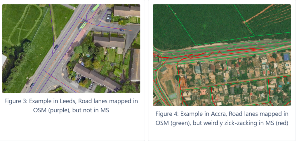
Road Lanes
It often happens that the two directions of a road are mapped as separate features in OSM , while in MS roads there is just a single line feature representing the road.
This leads to another phenomenon: The length of OSM roads overlaid by MS roads is bigger than the total length of the MS data itself. For example, 10 meter of MS roads might actually represent 20 meters of OSM roads.
To some extent this explains the limitations of Method 1: Length Comparison. Converting bi-directionally mapped roads into single-feature roads might resolve this issue.
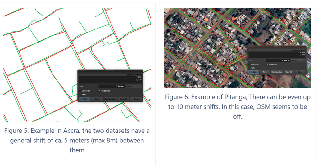
Misalignment of datasets
In general, we found that there is always a slight misalignment probably due to differences in the utilized satellite and remote sensing data. In some cities, the shift in roads of the data is very low (Heidelberg, Guatemala, Leeds). In other cities it is quite large (Accra, Pitanga). (Better understanding the disparities between regions of the world might make for an interesting analysis in itself.)
This misalignment of both datasets will have an effect on the Overlap Indicator A and B. Based on our observations, 5 to 8 meters might be good buffer sizes to start, but depending on the shift between datasets the buffer size might have to be regionally adapted.
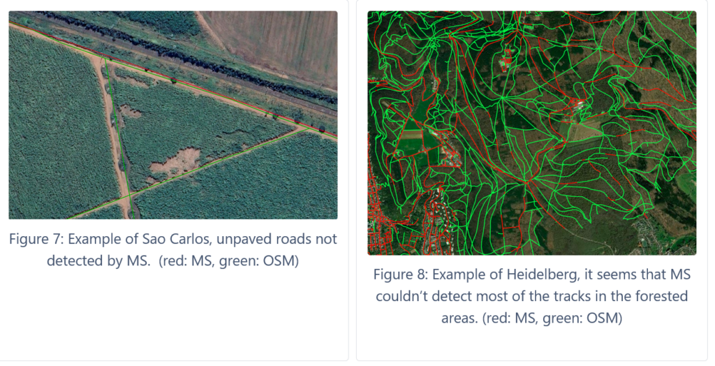
Missing roads in MS dataset
In general, we have realized that there are many false negatives (missing roads) in the MS dataset. It seems that unpaved roads and roads covered by trees are often not detected.
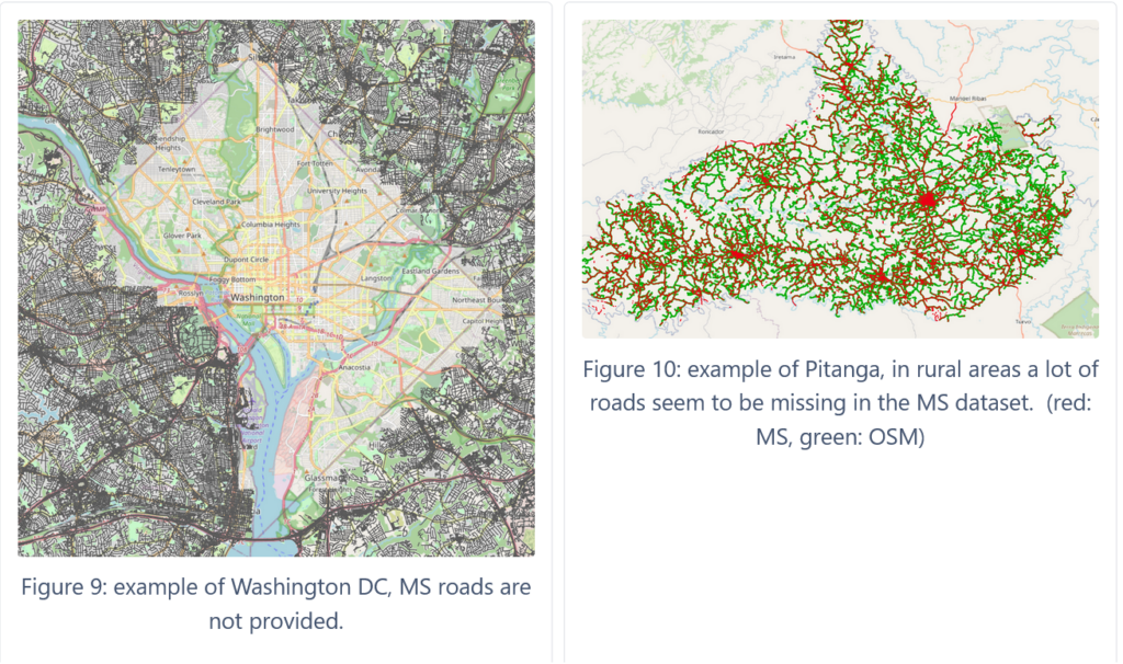
Missing roads in the MS dataset will have an effect on the results for Method 1: Length Comparison Method 3: Overlap Indicator B. Whereas it is difficult to account for these missing roads, this is affecting rural areas much stronger than urban areas. In some places such as Washington DC, MS roads are not available at all. It’s not clear if there are other regions which have been excluded systematically from the MS dataset.
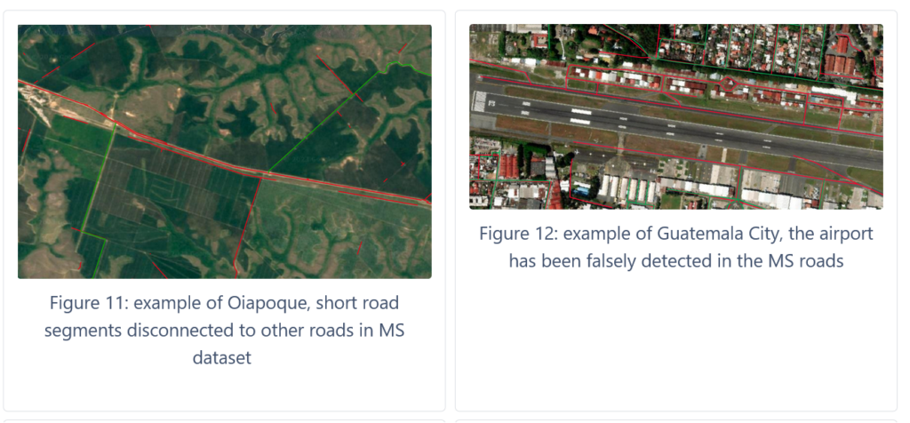
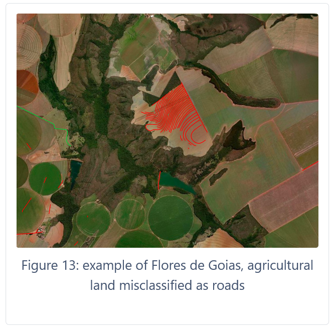
Misclassifications in MS dataset
Especially in rural areas, we have found various examples of false positive road detection in the MS dataset. Often they appear as very short roads, which are not connected to other parts of the MS road network. Sometimes other features, such as train tracks or runways at airports, have been wrongly identified as roads.
These misclassifications are mainly a problem for Method 1: length comparison and Method 2: Overlap Indicator A. It would be beneficial to apply some filtering to the MS datasets to remove these misclassifications.
Next Steps and Open Questions
These are only some first steps towards developing a better understanding of the value of the MS roads data for OSM data quality analysis. We have learned that there are still many open questions, which we need to tackle, so that we can provide a reliable completeness estimate for the OSM road network.
- How can we combine both overlap methods?
- To what extent are limitations of our experiment particular to certain geographic regions (e.g. countries) or characteristics (e.g. cities, rural areas, forests, desert, …)?
- What can be done to improve road data quality estimates especially for rural areas?
- To what extent does the selection of highway types influence the analysis results?
In addition, we would like to explore other datasets as well. As deep learning approaches are rapidly improving nowadays, we expect that more datasets will become available soon. A combination of several road layers might very likely overcome some of the limitations we have observed for the current version of MS roads.
Ultimately, our goal is to provide data quality indicators which can be easily accessed and calculated for all regions across the globe through the ohsome dashboard. If you are interested in this topic, you are welcome to send us any feedback via e-mail (ohsome@heigit.org).